Everyone likes to have a safety net, and scientists are no different. This month I will be discussing internal standards and how we can use them not only to improve the quality of our data, but also give us some ‘wiggle room’ when it comes to variation in sample preparation. Internal standards are widely used in every type of chromatographic analysis, so it is not surprising that their use also applies to common cannabis analyses. In my last article, I wrapped up our discussion of calibration and why it is absolutely necessary for generating valid data. If our calibration is not valid, then the label information that the cannabis consumer sees will not be valid either. These consumers are making decisions based on that data, and for the medical cannabis patient, valid data is absolutely critical. Internal standards work with calibration curves to further improve data quality, and luckily it is very easy to use them.
So what are internal standards? In a nutshell, they are non-analyte compounds used to compensate for method variations. An internal standard can be added either at the very beginning of our process to compensate for variations in sample prep and instrument variation, or at the very end to compensate only for instrument variation. Internal standards are also called ‘surrogates’, in some cases, however, for the purposes of this article, I will simply use the term ‘internal standard.’
Now that we know what internal standards are, let’s look at how to use them. We use an internal standard by adding it to all samples, blanks, and calibrators at the same known concentration. By doing this, we now have a single reference concentration for all response values produced by our instrument. We can use this reference concentration to normalize variations in sample preparation and instrument response. This becomes very important for cannabis pesticide analyses that involve lots of sample prep and MS detectors. Figure 1 shows a calibration curve plotted as we saw in the last article (blue diamonds), as well as the response for an internal standard added to each calibrator at a level of 200ppm (green circles). Additionally, we have three sample results (red triangles) plotted against the calibration curve with their own internal standard responses (green Xs).
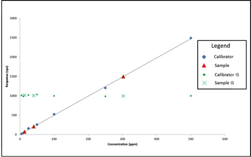
Figure 1: Calibration Curve with Internal Standard Responses and Three Sample Results
In this case, our calibration curve is beautiful and passes all of the criteria we discussed in the previous article. Lets assume that the results we calculate for our samples are valid – 41ppm, 303ppm, and 14ppm. Additionally, we can see that the responses for our internal standards make a flat line across the calibration range because they are present at the same concentration in each sample and calibrator. This illustrates what to expect when all of our calibrators and samples were prepared correctly and the instrument performed as expected. But lets assume we’re having one of those days where everything goes wrong, such as:
- We unknowingly added only half the volume required for cleanup for one of the samples
- The autosampler on the instrument was having problems and injected the incorrect amount for the other two samples
Figure 2 shows what our data would look like on our bad day.
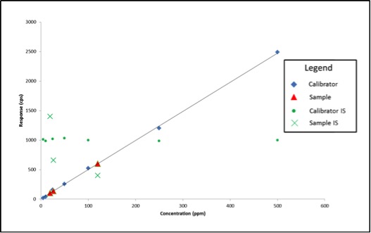
Figure 2: Calibration Curve with Internal Standard Responses and Three Sample Results after Method Errors
We experienced no problems with our calibration curve (which is common when using solvent standard curves), therefore based on what we’ve learned so far, we would simply move on and calculate our sample results. The sample results this time are quite different: 26ppm, 120ppm, and 19ppm. What if these results are for a pesticide with a regulatory cutoff of 200ppm? When measured accurately, the concentration of sample 2 is 303ppm. In this example, we may have unknowingly passed a contaminated product on to consumers.
In the first two examples, we haven’t been using our internal standard – we’ve only been plotting its response. In order to use the internal standard, we need to change our calibration method. Instead of plotting the response of our analyte of interest versus its concentration, we plot our response ratio (analyte response/internal standard response) versus our concentration ratio (analyte concentration/internal standard concentration). Table 1 shows the analyte and internal standard response values for our calibrators and samples from Figure 2.
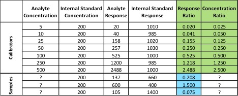
Table 1: Values for Calibration Curve and Samples Using Internal Standard
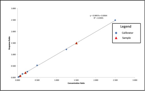
Figure 3: Calibration Curve and Sample Results Calculated Using Internal Standard Correction
We can see that our axes have changed for our calibration curve, so the results that we calculate from the curve will be in terms of concentration ratio. We calculate these results the same way we did in the previous article, but instead of concentrations, we end up with concentration ratios. To calculate the sample concentration, simply multiply by the internal standard amount (200ppm). Figure 4 shows an example calculation for our lowest concentration sample.
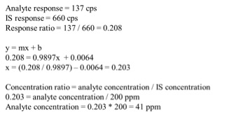
Figure 4: Example Calculation for Sample Results for Internal-Standard Corrected Curve
Using the calculation shown in Figure 4, our sample results come out to be 41ppm, 302ppm, and 14ppm, which are accurate based on the example in Figure 1. Our internal standards have corrected the variation in our method because they are subjected to that same variation.
